
WGCNA学习:WGCNA分析实战
1.WGCNA安装
> install.packages("BiocManager")
> BiocManager::install("WGCNA")
> library(WGCNA)
2.数据准备与读入
2.1数据准备
需要两个数据
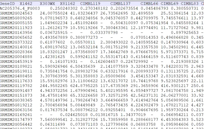
表达矩阵(All_fpkm.list)
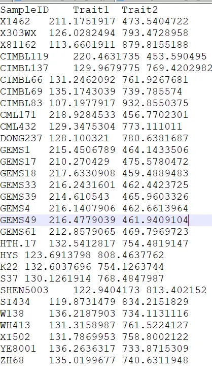
表型文件(pheno.txt),需要注意表型文件分为两类,连续变量型与分类变量型。
2.2 数据读入
library(WGCNA)
library(reshape2)
library(stringr)
setwd('D:/data/wgcna/Categorical')
options(stringsAsFactors = T)# 在读入数据时,遇到字符串后,将其转换成因子,连续型变量要改为FALSE
enableWGCNAThreads()#打开多线程
##====================step 1 :数据读入
RNAseq_voom <- fpkm

## 因为WGCNA针对的是基因进行聚类,而一般我们的聚类是针对样本用hclust即可,所以这个时候需要转置
WGCNA_matrix = t(RNAseq_voom[order(apply(RNAseq_voom,1,mad), decreasing = T)[1:5000],])
datExpr <- WGCNA_matrix  ## top 5000 mad genes

#明确样本数和基因
nGenes = ncol(datExpr)
nSamples = nrow(datExpr)
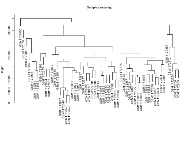
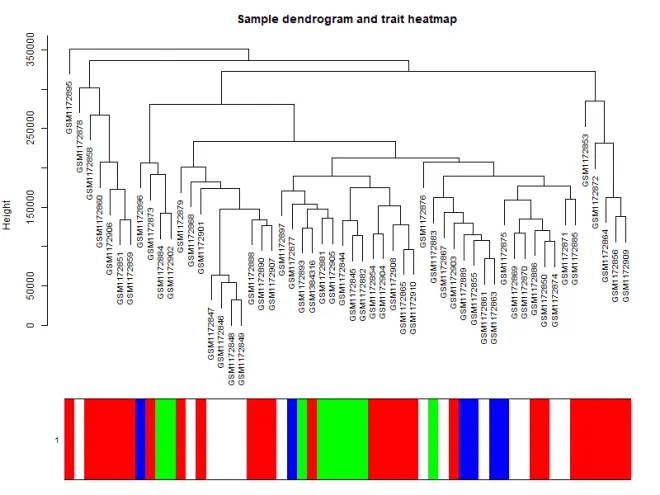
#首先针对样本做个系统聚类
datExpr_tree<-hclust(dist(datExpr), method = "average")
par(mar = c(0,5,2,0))
png("img/step1-sample-cluster.png",width = 800,height = 600)
plot(datExpr_tree, main = "Sample clustering", sub="", xlab="", cex.lab = 2,
       cex.axis = 1, cex.main = 1,cex.lab=1)
dev.off()
3. β值估计
##====================step 2:β值确定====
datExpr[1:4,1:4]
powers = c(c(1:10), seq(from = 12, to=20, by=2))
#设置beta值的取值范围
sft = pickSoftThreshold(datExpr, RsquaredCut = 0.9,powerVector = powers, verbose = 5)
#设置网络构建参数选择范围,计算无尺度分布拓扑矩阵
png("img/step2-beta-value.png",width = 800,height = 600)
par(mfrow = c(1,2));
cex1 = 0.9;
# Scale-free topology fit index as a function of the soft-thresholding power
plot(sft$fitIndices[,1], -sign(sft$fitIndices[,3])*sft$fitIndices[,2],
         xlab="Soft Threshold (power)",ylab="Scale Free Topology Model Fit,signed
R^2",type="n",
main = paste("Scale independence"));
text(sft$fitIndices[,1], -sign(sft$fitIndices[,3])*sft$fitIndices[,2],
        labels=powers,cex=cex1,col="red");
# this line corresponds to using an R^2 cut-off of h
abline(h=0.90,col="red")
# Mean connectivity as a function of the soft-thresholding power
plot(sft$fitIndices[,1], sft$fitIndices[,5],xlab="Soft Threshold (power)",ylab="Mean Connectivity", type="n",main = paste("Mean connectivity"))
text(sft$fitIndices[,1], sft$fitIndices[,5], labels=powers, cex=cex1,col="red")
dev.off()
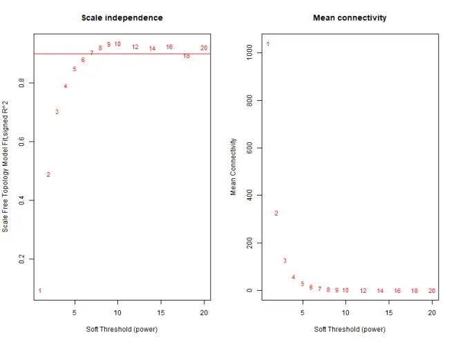
可以确定最佳β值为6
4. 一步法构建共表达矩阵
最核心的一步,同时也是最耗费计算资源的一步
##====================step 3:自动构建WGCNA模型==================
# 首先是一步法完成网络构建
net = blockwiseModules(
  datExpr,
  power = sft$powerEstimate,             #软阈值,前面计算出来的
  maxBlockSize = 6000,                   #最大block大小,将所有基因放在一个block中
  TOMType = "unsigned",                  #选择unsigned,使用标准TOM矩阵
  deepSplit = 2, minModuleSize = 30,     #剪切树参数,deepSplit取值0-4
  mergeCutHeight = 0.25,                 # 模块合并参数,越大模块越少
  numericLabels = TRUE,                  # T返回数字,F返回颜色
  pamRespectsDendro = FALSE,
  saveTOMs = TRUE,
  saveTOMFileBase = "FPKM-TOM",
  loadTOMs = TRUE,
  verbose = 3)
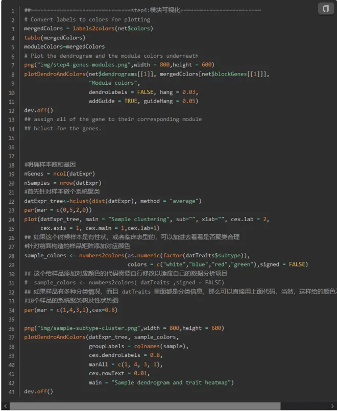
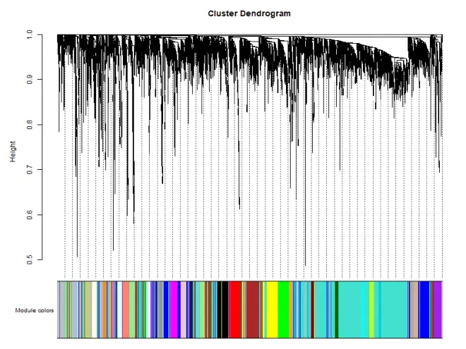
5. 模块可视化
可以看到模块用不同的颜色来标注,灰色模块是无法归类于任何模块的基因,在后续分析的时候不需要考虑
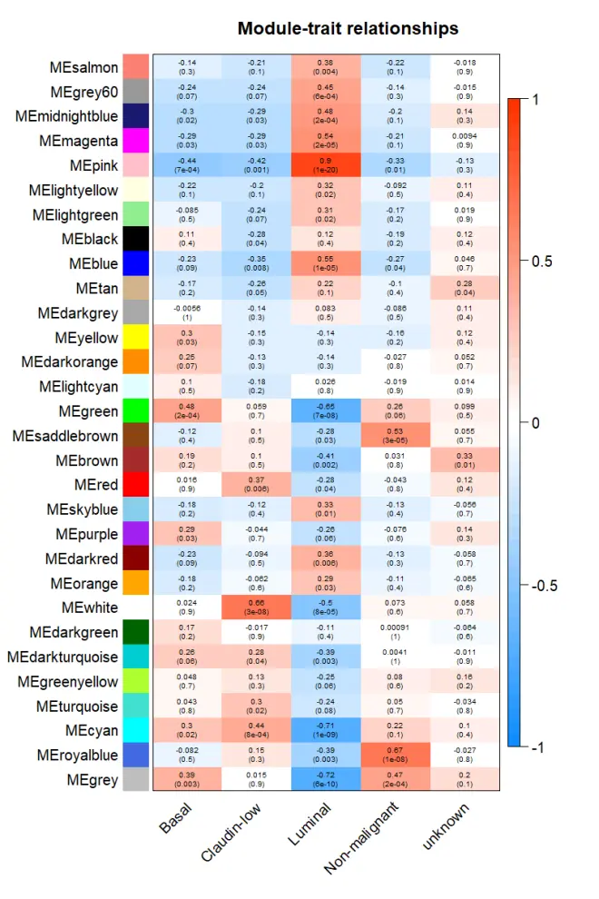
6.模块与性状的关系
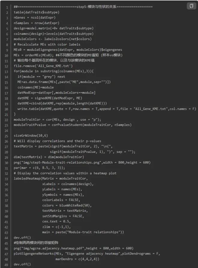
可以看到不同的模块与不同的性状是有不同的相关性的,在后续分析的时候我们可以选择感兴趣的模块进行分析。
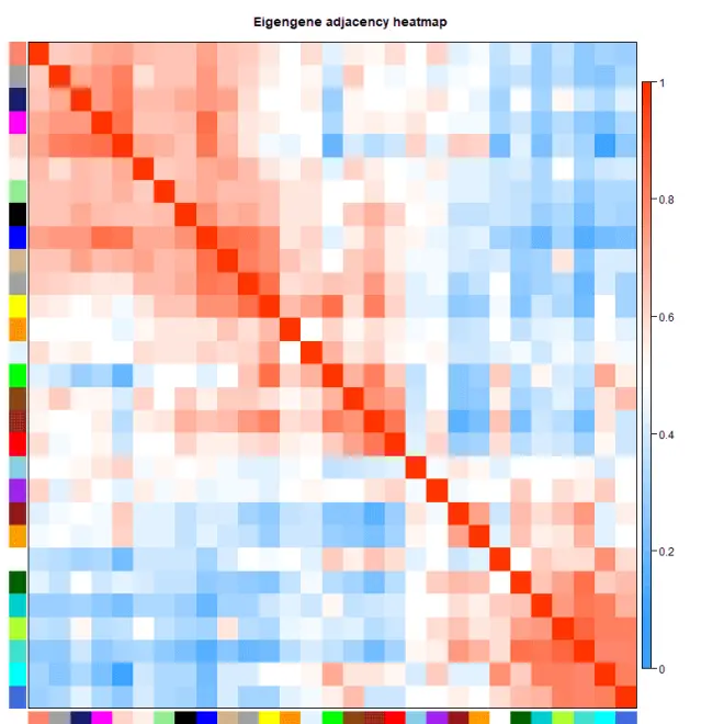
两两模块之间的邻接矩阵,主要看不同模块之间的相关性
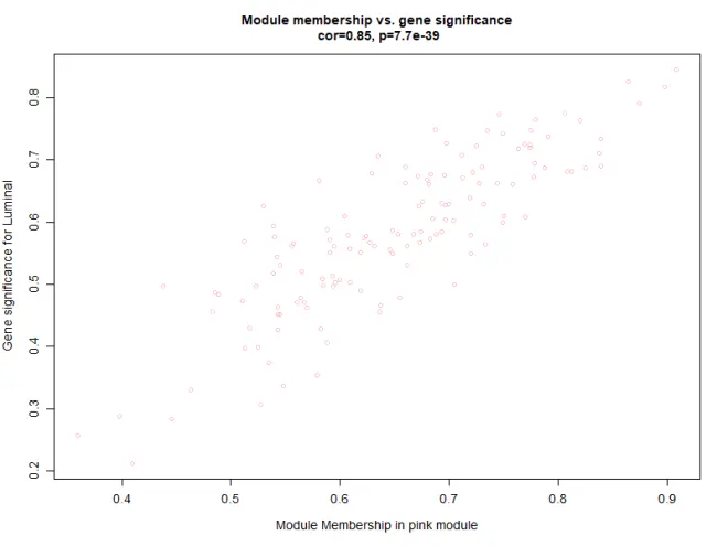
7. 选择感兴趣的模块进行分析
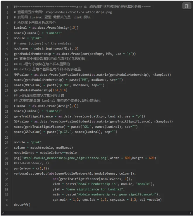
由于是分类变量,只能按照0至1量化,可以看出模块内的基因与表型有很好的线性关系
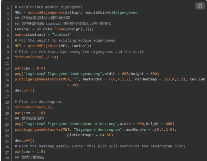
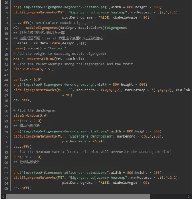
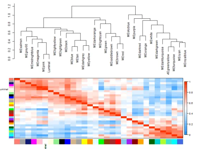
然后再绘制性状与模块的关系
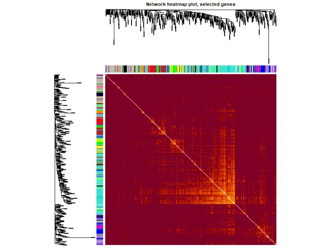
8.网络的可视化
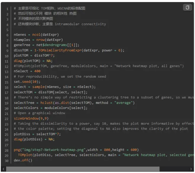
不知道为啥,这张图有点奇怪
9. 模块的导出
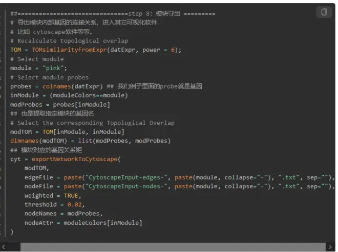
模块导出后可以用cytoscape构建网络,后面的教程会教大家利用这个文件构建网络图
后记
本次WGCNA的代码结合了生信技能树和PlantTech的WGCNA教程,原始数据也来自这两个教程,我将代码和原始数据上传到自己的github中,其中PlantTech课程是收费课程,我已将其下载,大家有需要可以去百度云下载
视频压缩包解压密码是我博客about界面下的一行小字(出自《蒲公英女孩》,标点是英文),如果链接炸了去博客找我联系方式。
github:https://github.com/Bioinformatics-rookie
blog:https://www.zhouxiaozhao.cn/
