By: Tao Steven Zheng (郑涛)

This article was originally posted on Brilliant.org and the Math & Physics Wikia by the same author.

From Wave to Particle

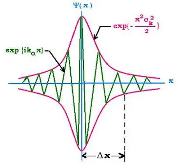
Louis de Broglie taught us that all particles in the universe possess a wavelength. We will consider microscopic objects because they closely follow the wave-particle duality more than macroscopic objects. Consider a particle travelling in space with no potential to hold it down: we will call this the free particle. Since microscopic particles also behave like waves, we will model the free particle as a sinusoidal plane wave enveloped in a corresponding wave-packet. The sinusoidal plane wave propagates in space and evolves in time; thus, we can express it as a complex exponential function

and wave-packet (Figure 1) 

Using de Broglie’s equations of momentum and energy , we can rewrite the wave-packet equation as

What can we do with this integral so that we can describe a physical system? Why not take derivatives until two sides of an equation match? Let’s begin by taking the time derivative and two derivatives in space:

Now there is one final step to do: balancing. If we multiply the time derivative by and the second spatial derivative by , we get

It is customary in physics to describe physical systems in terms of total energy, which is the sum of the kinetic and potential energies. So all we have to do to this free particle is add to the right-hand side. Hence, 

The equation uncovered above is the Schrödinger equation for a single non-relativistic particle in one spatial dimension!

Operators

Linear algebra, more specifically linear operator algebra, is the language of quantum mechanics. Thus, it is most appropriate to write the Schrödinger equation in operator form. An operator is an instruction that acts on a function. An operator is linear if it satisfies the identity

where are scalars. This is where quantum mechanics starts to get abstract, so I will introduce some concrete examples. Consider the operators and . If we act on some position quantity , we get the differential . Hence, momentum is a differential operator. Looks straightforward enough! But consider the convenient things we can do to operators, for example: becomes .

Now let us look at the Schrödinger equation in operator form:

For the time-independent case , we replace the time derivative term with total energy, and if we want to be even more compact, we may denote the operator on the right-hand side with the Hamiltonian operator 

Notice how this is shorter? Well, that's good and all, but not the point. The point is that we are acting a Hamiltonian operator on the wavefunction <math> \Psi </math>, which is convenient for reasons unclear at the moment. You see, linear operators can describe many things, but all linear operators follow the same algebra. We have entered the realm where abstract algebra infiltrates all of physics for the convenience of problem solving. So from now on, we will consider operators to act on physical quantities and objects.

Determinate States

When you solve the time-independent Schrödinger equation, you will encounter values of energy that satisfy

These are called determinate states, which are eigenfunctions (also called eigenstates) of the linear operator with corresponding energy eigenvalues . When a linear operator possesses several eigenvalues, we call the set of eigenvalues its spectrum. If two or more linearly independent eigenfunctions share the same eigenvalue, we call those spectra degenerate. You will later learn that degeneracies play an important role in describing the atom; hence much of quantum chemistry and solid-state physics.

Problems

1. Dispersion Relation

Use the de Broglie relations to obtain the dispersion relation of wave-packets. [Hint:  is proportional to .]

2. One Dimensional Particle in a Box - Part 1

Consider the potential that is 0 within the region and infinite elsewhere. Solve the time-independent Schrödinger equation for this potential with boundary conditions: . Once you find the wavefunction (solution), normalize the wavefunction . [Note: is just .]    

3.One Dimensional Particle in a Box - Part 2

Now that you have found the solution to the 1D Particle in a Box, find the set of permissible eigenenergies (energy levels). Remember that the wavenumber of a matter-wave is given by where . This will help you simplify .