
Lab Exercise 2
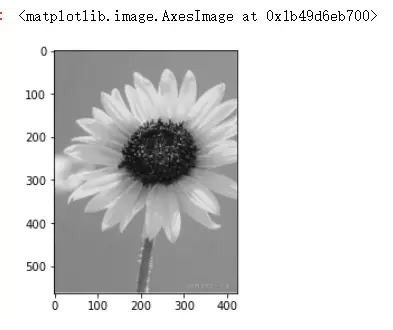
1. Select an interesting image, design a binarization rule (which can be a simple threshold or other complex functions), binarize the image, and display the original image and the binary image. Briefly explain the binarization rule and the result you obtained.
2. Select a picture (the size must be greater than 1024*1024), this question can be completed by calling the third-party functions. At the same time, I also encourage capable students to write their own implementation from scratch:
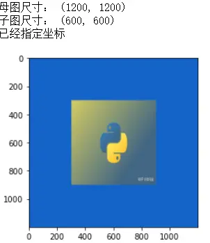
1) Resize the image to half the width and height, but keep the original size of the canvas, and the resized image should be centered (the resized image and canvas share the same center). All pixels on the canvas should be set to blue. Plot the result.
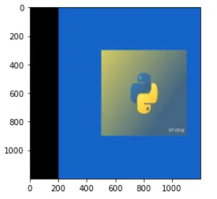
2) Based on the result of 1), move the resized image by 200 pixels in the positive direction of the x-axis, and plot the result.
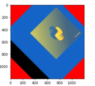
3) Based on the result of 2), Rotate the image (don't rotate canvas) 45 degrees counter-clockwise along the positive direction of the z-axis (pointing out screen) via the the center of the picture (not the center of the canvas), and plot the result.
3. Histogram Equalization
1) Students are required to write your own code from scratch (Calling third-party functions to complete histogram, cumulative histogram, and equalization calculations are not allowed): to implement a single-channel histogram function, a single-channel cumulative histogram function and a single-channel histogram equalization function.
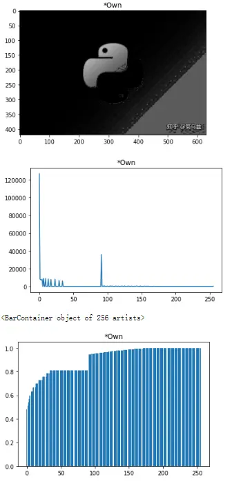
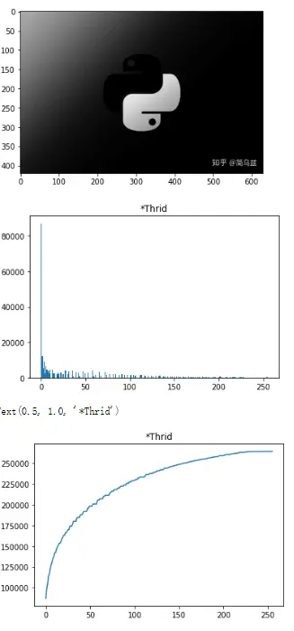
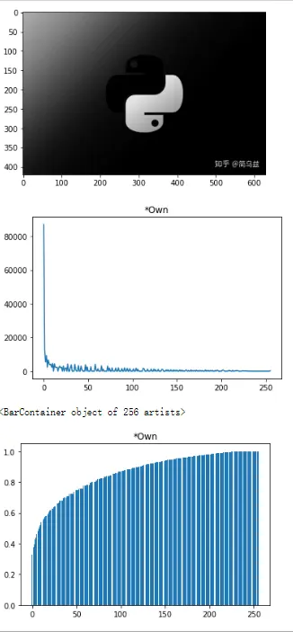
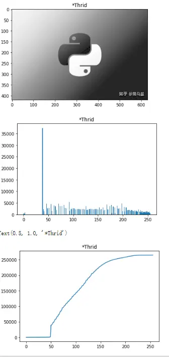
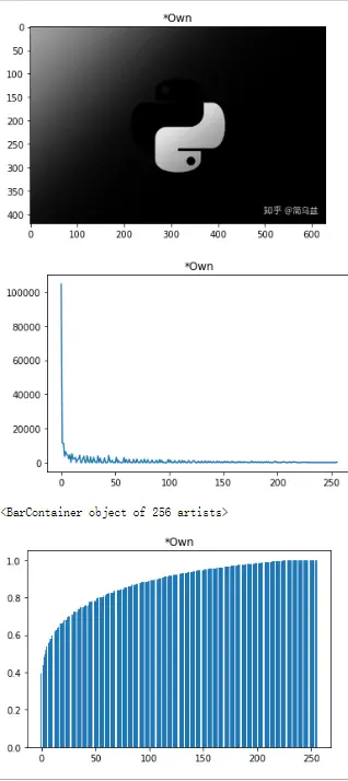
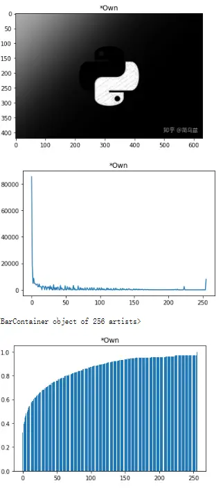
2) Select any color image, and perform histogram equalization on its channels respectively. For each channel, display the original image, histogram, and cumulative histogram before equalization, as well as after equalization.
More specifically, 12 images for each channel are required to be plotted and arranged in the following way:
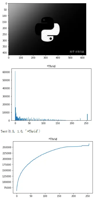
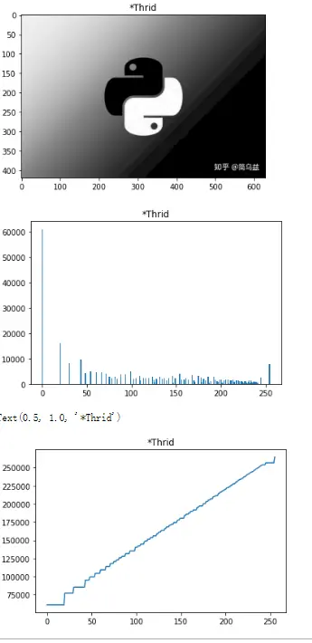
*Third indicates that the result is generated by calling the third party function.
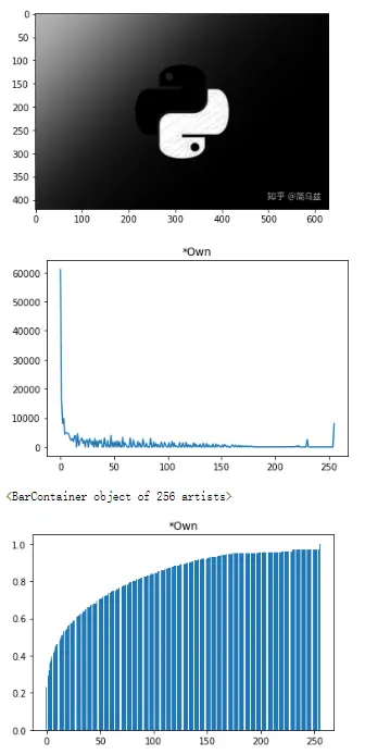
*Own indicates that the result must be generated by calling your own function implemented in 1).
Original image (e.g. Red channel), Histogram (*Third), Cumulative Histogram (*Third)
Original image (e.g. Red channel), Histogram (*Own), Cumulative Histogram (*Own)
Equalized Image (*Third), Histogram (*Third), Cumulative Histogram (*Third)
Equalized Image(*Own), Histogram (*Own), Cumulative histogram (*Own)
There should be 36 images in total for three channels.
3) Analyze your results and compare your results with third-party results. Are they consistent with each other? If not, please explain why there are differences.
作答(仅供参考,并不是对的)
import CV2 as cv
import numpy as np
import matplotlib.pyplot as plt
from PIL import Image
import matplotlib.image as imag
import os
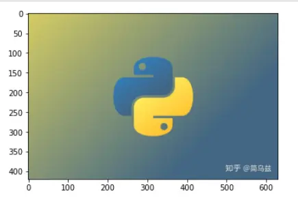
img=cv.imread("image/cda4671f75fb49c584d4332e76e7bf21.png")
plt.imshow(img)
二值化
def two_value(image):
gray = cv.cvtColor(image, cv.COLOR_BGR2GRAY) ##要二值化图像,必须先将图像转为灰度图
ret, binary = cv.threshold(gray, 0, 255, cv.THRESH_BINARY | cv.THRESH_OTSU)
cv.imwrite("image/two_value.png",binary)
cv.waitKey(0)
cv.destroyAllWindows()
def show(img):
if img.ndim==2:
plt.imshow(img,cmap='gray')
else:
plt.imshow(cv.cvtColor(img,cv.COLOR_BGR2RGB))
plt.show()
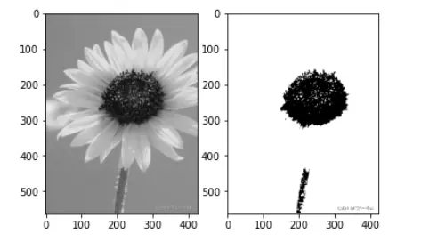
two_value(img)
test=cv.imread("image/two_value.png")
plt.figure()#创建画布
plt.subplot(1,2,1)
plt.imshow(img)
plt.subplot(1,2,2)
plt.imshow(test)
plt.show()
对第一题的解释
直接写一个函数来转换,使用cv里的函数,我这里是直接读取的灰值图像,然后对灰值图像进行处理,使用cv的threshold 函数来及逆行全局阙值的处理, 参数的意思是THRESH_BINARY 超过阈值的值为最大值,其他值是0。CV2.THRESH_OTSU使用最小二乘法处理像素点,而CV2.THRESH_TRIANGLE使用三角算法处理像素点。这样超过阙值的是255 低于阙值的是黑色,实现二值化。得到的结果中,黑色被大量保留,其他则变为白色
第二题
img2=cv.imread("image/e1c0cfd9e202882aefe6fc5ae89be447.png")
np.shape(img2)
#对图片进行修改尺寸
size=(1200,1200)
img2_new=cv.resize(img2,size)
#那么如何手写修改尺寸呢
show(img2_new)
#缩小图片,但保持画布的大小不变,使用蓝色填充
hight,width=img2_new.shape[:2]
size=(600,600)
img2_new=cv.resize(img2,size)
img2_new=cv.cvtColor(img2_new,cv.COLOR_BGR2RGB)
img2_new=Image.fromarray(img2_new)
img2_new.save("img2_new.png")
#创建一个画布,蓝色,然后把缩小的图片放到中间
def InitCanvasV3(width, height, color=(255, 255, 255)):
canvas = np.ones((height, width, 3), dtype="uint8")
canvas[:] = color
return canvas
def blend_two_images2(img1,img2):
img1 = img1.convert('RGBA')
img2 = img2.convert('RGBA')
r, g, b, alpha = img2.split()
alpha = alpha.point(lambda i: i>0 and 204)
img = Image.composite(img2, img1, alpha)
img.show()
img.save( "image/blend2.png")
# 初始化一个蓝色的画布
canvas_color = InitCanvasV3(1200, 1200, color=(20, 100, 200))
#先保存
canvas_color=Image.fromarray(canvas_color)
canvas_color.save("canvas_color.png")
canvas_color=Image.open("canvas_color.png")
def Picture_Synthesis(M_Img,
S_Img,
save_img,
coordinate=None):
"""
:param mother_img: 母图
:param son_img: 子图
:param save_img: 保存图片名
:param coordinate: 子图在母图的坐标
:return:
"""
#将图片赋值,方便后面的代码调用
factor = 1#子图缩小的倍数1代表不变,2就代表原来的一半
#给图片指定色彩显示格式
M_Img = M_Img.convert("RGBA") # CMYK/RGBA 转换颜色格式(CMYK用于打印机的色彩,RGBA用于显示器的色彩)
# 获取图片的尺寸
M_Img_w, M_Img_h = M_Img.size # 获取被放图片的大小(母图)
print("母图尺寸:",M_Img.size)
S_Img_w, S_Img_h = S_Img.size # 获取小图的大小(子图)
print("子图尺寸:",S_Img.size)
size_w = int(S_Img_w / factor)
size_h = int(S_Img_h / factor)
# 防止子图尺寸大于母图
if S_Img_w > size_w:
S_Img_w = size_w
if S_Img_h > size_h:
S_Img_h = size_h
# # 重新设置子图的尺寸
# icon = S_Img.resize((S_Img_w, S_Img_h), Image.ANTIALIAS)
icon = S_Img.resize((S_Img_w, S_Img_h), Image.ANTIALIAS)
w = int((M_Img_w - S_Img_w) / 2)
h = int((M_Img_h - S_Img_h) / 2)
try:
if coordinate==None or coordinate=="":
coordinate=(w, h)
# 粘贴子图到母图的指定坐标(当前居中)
M_Img.paste(icon, coordinate, mask=None)
else:
print("已经指定坐标")
# 粘贴子图到母图的指定坐标(当前居中)
M_Img.paste(icon, coordinate, mask=None)
except:
print("坐标指定出错 ")
# 保存图片
M_Img.save(save_img)
Picture_Synthesis(canvas_color,img2_new,save_img="image/newimg.png",coordinate=(300,300))
image_new=cv.imread("image/newimg.png")
show(image_new)
M = np.float32([[1, 0, 200], [0, 1, 0]])
shifted = cv.warpAffine(image_new, M, (width, hight))
show(shifted)
#3)根据2)的结果,通过画面中心(不是画布中心),将图像(不要旋转画布)沿z轴正方向(指向屏幕外)逆时针旋转45度,绘制结果。
test_3=cv.getRotationMatrix2D((width//2,hight//2),45,1)
image_rotation=cv.warpAffine(shifted,test_3,(width,hight),borderValue=(0,0,255))
show(image_rotation)
#实现单通道直方图函数、单通道累积直方图函数和单通道直方图均衡函数。
from os.path import isfile
from PIL import Image
import collections
import matplotlib.pyplot as plt
import numpy as np
import CV2 as cv
def show(img):
if img.ndim==2:
plt.imshow(img,cmap='gray')
else:
plt.imshow(cv.cvtColor(img,cv.COLOR_BGR2RGB))
plt.show()
#单通道直方图函数
#转成一维列表
def test_ravel(gray):
a=[]
for i in np.array(gray):
for y in i:
#这里已经拿到单个了,那么一唯列表
a.append(y)
return list(a)
#计算所欲灰度级
def test_Counter_gray(gray):
sum={}
for i in gray:
if(i in sum.keys()):
#存在
sum[i]+=1
else:
#不存在
sum[i]=1
return sum
#直方图函数
def clczhifangtu(gray) :
# gray=gray.convert('L')
hist_new = []
num = []
hist_result = []
hist_key = []
gray1 = test_ravel(gray)
obj = test_Counter_gray(gray1)
# print(obj)
obj = sorted(obj.items(),key=lambda item:item[0])
for each in obj :
hist1 = []
key = list(each)[0]
each =list(each)[1]
hist_key.append(key)
hist1.append(each)
hist_new.append(hist1)
#检查从0-255每个通道是否都有个数,没有的话添加并将值设为0
for i in range (0,256) :
if i in hist_key :
num = hist_key.index(i)
hist_result.append(hist_new[num])
else :
hist_result.append([0])
if len(hist_result) < 256 : #检查循环后的列表中是不是已经包含所有的灰度级
for i in range (0,256-len(hist_result)) :
hist_new.append([0])
# hist_result = np.array(hist_result)
#这里不用np.array 会发生什么,都是数组
# print(hist_result)
return hist_result
im = Image.open('image/e1c0cfd9e202882aefe6fc5ae89be447.png')
im=im.convert('L')
# print(type(im))
# print(np.array(im))
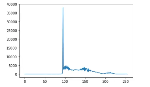
y=clczhifangtu(im)#y已经统计好区间了
# print(y)
plt.plot(y)
plt.show()
# print(np.array(im).ravel())
# test_ravel(im)
#单通道累计直方图函数
def histogram_sum(gray):#绘制累计直方图
# cdf=clczhifangtu(gray)
# cdf = 255.0 * cdf / cdf[-1]
try:
x = gray.size[0]
y = gray.size[1]
except:
#对于是从open过来的函数
gray= Image.fromarray(gray)
x = gray.size[0]
y = gray.size[1]
ret = np.zeros(256)
#如果不满足则转型呀
try:
for i in range(x):
for j in range(y):
k = gray.getpixel((i,j))#正常捕获像素值
ret[k] = ret[k ]+1
except:
#numpy.array捕获像素值
# gray= Image.fromarray(gray)
for i in range(x):
for j in range(y):
k = gray.getpixel((i,j))#正常捕获像素值
ret[k] = ret[k]+1
# print(type(gray)) <class 'PIL.Image.Image'>
for k in range(1,256):
ret[k] = ret[k]+ret[k-1]#累加
for k in range(256):
ret[k] = ret[k]/(x*y)
return ret
im = Image.open('image/e1c0cfd9e202882aefe6fc5ae89be447.png')
im=im.convert('L')
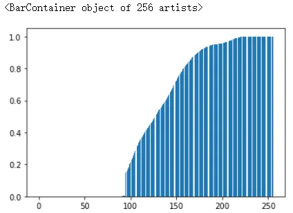
plt.figure()
plt.bar(range(256),histogram_sum(im))#描绘柱状图
# histogram_sum(im)
# sum=0
# for i in clczhifangtu(im):
# sum+=i
# 单通道直方图均衡化
def probability_to_histogram(img, prob):
# img.convert('L')
# 根据像素概率将原始图像直方图均衡化
# :param img:
# :param prob:
# :return: 直方图均衡化后的图像
prob=histogram_sum(img)
img_map = [int(i * prob[i]) for i in range(256)] # 像素值映射#这里只是一个一唯的数组
# 像素值替换
# print(img)
# print(img_map[1])
# img=np.array(img)
# print(img)
# print(img[1][1])
r, c = img.shape
for ri in range(r):
for ci in range(c):
img[ri, ci] = img_map[img[ri, ci]]
return img
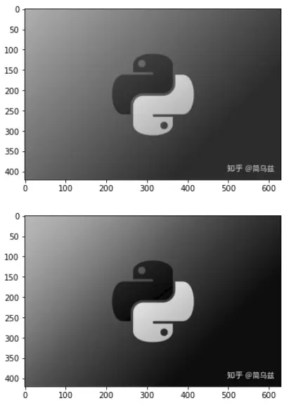
img3=cv.imread("image/e1c0cfd9e202882aefe6fc5ae89be447.png", cv.IMREAD_GRAYSCALE)
show(img3)
pro_img=probability_to_histogram(img3,clczhifangtu(img3))
show(pro_img)
# 上面是测试
img_t=cv.imread("image/e1c0cfd9e202882aefe6fc5ae89be447.png")
show(img_t)
# 通道分离
b,g,r = cv.split(img_t)
# cv.imshow("Blue",r)
# cv.imshow("Red",g)
# cv.imshow("Green",b)
# cv.waitKey(0)
# cv.destroyAllWindows()
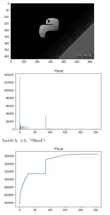
b 通道 均衡化前
# 原始图像
show(b)
#直方图
plt.hist(b.ravel(), 256)
plt.title('*Thrid')
plt.show()
# 累积直方图
hist_img, _ = np.histogram(b, 256)
cdf_img = np.cumsum(hist_img) # accumulative histogram
plt.plot(range(256), cdf_img)
plt.title('*Thrid')
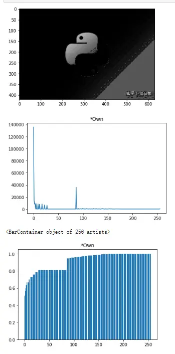
# 原始图像
show(b)
# 直方图
y=clczhifangtu(b)
plt.plot(y)
plt.title("*Own")
plt.show()
#累积直方图
plt.figure()
plt.title("*Own")
plt.bar(range(256),histogram_sum(b))#描绘柱状图
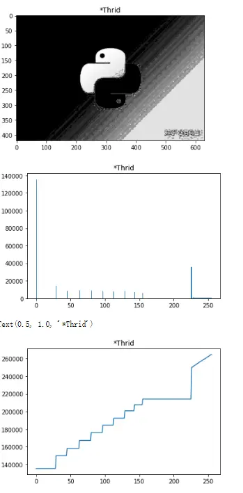
b 通道 均衡化后
# 均衡图像(*Third),直方图(*Third),累积直方图(*Third)
#直方图均衡化处理
result = cv.equalizeHist(b)
plt.title('*Thrid')
show(result)
#直方图
plt.hist(result.ravel(), 256)
plt.title('*Thrid')
plt.show()
# 累积直方图
hist_img, _ = np.histogram(result,256)
cdf_img = np.cumsum(hist_img) # accumulative histogram
plt.plot(range(256), cdf_img)
plt.title('*Thrid')
pro_img=probability_to_histogram(b,clczhifangtu(b))
plt.title("*Own")
show(pro_img)
# 直方图
y=clczhifangtu(pro_img)
plt.plot(y)
plt.title("*Own")
plt.show()
#累积直方图
plt.figure()
plt.title("*Own")
plt.bar(range(256),histogram_sum(pro_img))#描绘柱状图
g通道 均衡化前
# 原始图像
show(g)
#直方图
plt.hist(g.ravel(), 256)
plt.title('*Thrid')
plt.show()
# 累积直方图
hist_img, _ = np.histogram(g, 256)
cdf_img = np.cumsum(hist_img) # accumulative histogram
plt.plot(range(256), cdf_img)
plt.title('*Thrid')
# 原始图像
show(g)
# 直方图
y=clczhifangtu(g)
plt.plot(y)
plt.title("*Own")
plt.show()
#累积直方图
plt.figure()
plt.title("*Own")
plt.bar(range(256),histogram_sum(g))#描绘柱状图
g通道 均衡化后
# 均衡图像(*Third),直方图(*Third),累积直方图(*Third)
#直方图均衡化处理
result = cv.equalizeHist(g)
plt.title('*Thrid')
show(result)
#直方图
plt.hist(result.ravel(), 256)
plt.title('*Thrid')
plt.show()
# 累积直方图
hist_img, _ = np.histogram(result,256)
cdf_img = np.cumsum(hist_img) # accumulative histogram
plt.plot(range(256), cdf_img)
plt.title('*Thrid')
pro_img=probability_to_histogram(g,clczhifangtu(g))
plt.title("*Own")
show(pro_img)
# 直方图
y=clczhifangtu(pro_img)
plt.plot(y)
plt.title("*Own")
plt.show()
#累积直方图
plt.figure()
plt.title("*Own")
plt.bar(range(256),histogram_sum(pro_img))#描绘柱状图
r通道 均衡化前
# 原始图像
show(r)
#直方图
plt.hist(r.ravel(), 256)
plt.title('*Thrid')
plt.show()
# 累积直方图
hist_img, _ = np.histogram(r, 256)
cdf_img = np.cumsum(hist_img) # accumulative histogram
plt.plot(range(256), cdf_img)
plt.title('*Thrid')
# 原始图像
show(r)
# 直方图
y=clczhifangtu(r)
plt.plot(y)
plt.title("*Own")
plt.show()
#累积直方图
plt.figure()
plt.title("*Own")
plt.bar(range(256),histogram_sum(r))#描绘柱状图
r通道 均衡化后
# 均衡图像(*Third),直方图(*Third),累积直方图(*Third)
#直方图均衡化处理
result = cv.equalizeHist(r)
plt.title('*Thrid')
show(result)
#直方图
plt.hist(result.ravel(), 256)
plt.title('*Thrid')
plt.show()
# 累积直方图
hist_img, _ = np.histogram(result,256)
cdf_img = np.cumsum(hist_img) # accumulative histogram
plt.plot(range(256), cdf_img)
plt.title('*Thrid')
pro_img=probability_to_histogram(r,clczhifangtu(r))
plt.title("*Own")
show(pro_img)
# 直方图
y=clczhifangtu(pro_img)
plt.plot(y)
plt.title("*Own")
plt.show()
#累积直方图
plt.figure()
plt.title("*Own")
plt.bar(range(256),histogram_sum(pro_img))#描绘柱状图
分析结果并与之比较
直方图方面自己发函数与第三方函数相比较容易丢失数据或者处理不到位,产生偏差,统计的不到位,在直方图显示上,咱自己的函数大体没啥问题,主要是有些小灰度上统计不好,应该是把一些算到其他地方去了 累计直方图的话,除了表现形式不同,大体的趋势和精准度是差不多的
在均衡化方面,对于灰度级0的处理是不到位的,其他数级的分配是好的,总体能满足,但是依然有点瑕疵,应该对第一组数据进行详细在处理,不然达不到道理
