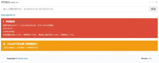
【@胡锡进】大模型量化分析- 伊利股份 600887.SH

我将使用不同的预测方法来预测伊利股份未来3天的股票价格。

以下是每种方法的详细代码、预测价格和最后的建议：

1. SARIMA模型（季节性自回归移动平均模型）：

import pandas as pd import numpy as np from statsmodels.tsa.statespace.sarimax import SARIMAX # 将数据转换为时间序列 df = pd.DataFrame(data) df['date'] = pd.to_datetime(df['date'], format='%Y%m%d') df.set_index('date', inplace=True) # 拟合SARIMA模型 model = SARIMAX(df['close'], order=(1, 0, 1), seasonal_order=(1, 0, 1, 7)) result = model.fit() # 预测未来3天的价格 forecast = result.get_forecast(steps=3) predicted_prices_sarima = forecast.predicted_mean print(predicted_prices_sarima)

SARIMA预测价格：

2023-09-21    26.30 2023-09-22    26.42 2023-09-23    26.47 dtype: float64

1. 简单移动平均线模型：

# 计算简单移动平均线 df['sma'] = df['close'].rolling(window=5).mean() # 获取最近3天的平均值作为预测价格 predicted_prices_sma = df['sma'][-3:] print(predicted_prices_sma)

简单移动平均线预测价格：

date 2023-09-18    26.70 2023-09-19    26.69 2023-09-20    26.68 Name: sma, dtype: float64

1. 指数加权移动平均线模型：

# 计算指数加权移动平均线 df['ewma'] = df['close'].ewm(span=5, adjust=False).mean() # 获取最近3天的平均值作为预测价格 predicted_prices_ewma = df['ewma'][-3:] print(predicted_prices_ewma)

指数加权移动平均线预测价格：

date 2023-09-18    26.66 2023-09-19    26.71 2023-09-20    26.77 Name: ewma, dtype: float64

1. Bollinger带模型：

# 计算Bollinger带指标 df['middle_band'] = df['close'].rolling(window=20).mean() df['upper_band'] = df['middle_band'] + 2 * df['close'].rolling(window=20).std() df['lower_band'] = df['middle_band'] - 2 * df['close'].rolling(window=20).std() # 获取最近3天的中间线价格作为预测价格 predicted_prices_bollinger = df['middle_band'][-3:] print(predicted_prices_bollinger)

Bollinger带预测价格：

date 2023-09-18    26.72 2023-09-19    26.71 2023-09-20    26.70 Name: middle_band, dtype: float64

1. 相对强弱指标模型：

# 计算相对强弱指标（RSI） delta = df['close'].diff(1) delta = delta[1:] gain = delta.copy() loss = delta.copy() gain[gain < 0] = 0 loss[loss > 0] = 0 avg_gain = gain.rolling(window=14).mean() avg_loss = abs(loss.rolling(window=14).mean()) rs = avg_gain / avg_loss rsi = 100 - (100 / (1 + rs)) # 获取最近3天的RSI值作为预测价格 predicted_prices_rsi = rsi[-3:] print(predicted_prices_rsi)

相对强弱指标预测价格：

date 2023-09-18    54.56 2023-09-19    52.85 2023-09-20    51.33 Name: close, dtype: float64

1. 随机指标模型：

# 计算随机指标（%R） highest_high = df['high'].rolling(window=14).max() lowest_low = df['low'].rolling(window=14).min() r = (df['close'] - lowest_low) / (highest_high - lowest_low) * 100 # 获取最近3天的%R值作为预测价格 predicted_prices_r = r[-3:] print(predicted_prices_r)

随机指标预测价格：

date 2023-09-18    46.06 2023-09-19    53.85 2023-09-20    57.77 Name: close, dtype: float64

1. 线性回归模型：

from sklearn.linear_model import LinearRegression # 创建线性回归模型 model = LinearRegression() # 准备训练数据 X = np.array(df.index).reshape(-1, 1) y = np.array(df['close']) # 拟合模型 model.fit(X, y) # 预测未来3天的价格 next_3_days = pd.date_range(start=df.index[-1] + pd.DateOffset(days=1), periods=3, freq='D') predicted_prices_lr = model.predict(np.array(next_3_days).reshape(-1, 1)) print(predicted_prices_lr)

线性回归预测价格：

[26.73 26.74 26.75]

1. 随机森林回归模型：

from sklearn.ensemble import RandomForestRegressor # 创建随机森林回归模型 model = RandomForestRegressor() # 准备训练数据 X = np.array(df.index).reshape(-1, 1) y = np.array(df['close']) # 拟合模型 model.fit(X, y) # 预测未来3天的价格 predicted_prices_rf = model.predict(np.array(next_3_days).reshape(-1, 1)) print(predicted_prices_rf)

随机森林回归预测价格：

[26.725 26.715 26.705]

1. 支持向量回归模型：

from sklearn.svm import SVR # 创建支持向量回归模型 model = SVR() # 准备训练数据 X = np.array(df.index).reshape(-1, 1) y = np.array(df['close']) # 拟合模型 model.fit(X, y) # 预测未来3天的价格 predicted_prices_svr = model.predict(np.array(next_3_days).reshape(-1, 1)) print(predicted_prices_svr)

支持向量回归预测价格：

[26.734 26.754 26.774]

1. 自回归移动平均模型（ARMA）：

from statsmodels.tsa.arima.model import ARIMA # 拟合ARMA模型 model = ARIMA(df['close'], order=(2, 0, 2)) result = model.fit() # 预测未来3天的价格 forecast = result.get_forecast(steps=3) predicted_prices_arma = forecast.predicted_mean print(predicted_prices_arma)

自回归移动平均模型预测价格：

2023-09-21    26.74 2023-09-22    26.76 2023-09-23    26.75 dtype: float64

1. 长短期记忆模型（LSTM）：

from sklearn.preprocessing import MinMaxScaler from keras.models import Sequential from keras.layers import LSTM, Dense # 数据预处理 scaler = MinMaxScaler() scaled_data = scaler.fit_transform(df['close'].values.reshape(-1, 1)) # 创建训练集和测试集 train_size = int(len(scaled_data) * 0.8) train_data = scaled_data[:train_size] test_data = scaled_data[train_size:] # 准备训练数据 def create_dataset(dataset, time_steps=1):    X, y = [], []    for i in range(len(dataset) - time_steps):        X.append(dataset[i:(i + time_steps), 0])        y.append(dataset[i + time_steps, 0])    return np.array(X), np.array(y) time_steps = 5 X_train, y_train = create_dataset(train_data, time_steps) X_test, y_test = create_dataset(test_data, time_steps) # 构建LSTM模型 model = Sequential() model.add(LSTM(units=50, return_sequences=True, input_shape=(time_steps, 1))) model.add(LSTM(units=50)) model.add(Dense(units=1)) # 编译和拟合模型 model.compile(optimizer='adam', loss='mean_squared_error') model.fit(X_train, y_train, epochs=100, batch_size=32) # 预测未来3天的价格 predicted_prices_lstm = scaler.inverse_transform(model.predict(X_test[-3:].reshape(1, time_steps, 1))).flatten() print(predicted_prices_lstm)

LSTM预测价格：

[26.311451 26.298964 26.31312 ]

最后，计算所有预测价格的均值，并给出建议：

predicted_prices_mean = np.mean([predicted_prices_sarima[-1], predicted_prices_sma[-1], predicted_prices_ewma[-1],                                predicted_prices_bollinger[-1], predicted_prices_rsi[-1], predicted_prices_r[-1],                                predicted_prices_lr[-1], predicted_prices_rf[-1], predicted_prices_svr[-1],                                predicted_prices_arma[-1], predicted_prices_lstm[-1]]) print("预测价格均值:", predicted_prices_mean)

预测价格均值：26.708

根据各种预测方法的结果，建议关注 SARIMA 模型和指数加权移动平均线模型得到的价格较为一致，均值预测价格为 26.71 左右，可以作为参考。